Adding game state to xR and xW

In previous blogs I have described how I used the speed of the ball, and its line and length to calculate the Expected Runs and Expected Wickets of that ball.  In this blog, I incorporate game state into these metrics, i.e. the over of the innings the ball was bowled.  The run rate, and indeed the probability of getting a wicket, is not constant throughout the course of a T20 innings.  Using data from nearly 4,000 T20 matches, we can calculate the average number of runs from each over of a innings, shown in the graph below.Teams generally have a bit of a go in the powerplay overs then completely start over in the 7th over – something I’ve always found a bit peculiar.  Usually, a spinner comes on and they knock him about in that over.  If teams target this over when the fielders have just recovered from the powerplay, perhaps they can increase their average scores by 2 or 3 runs – enough to win maybe 5% more games?  Anyway, the average number of runs then increases in a pretty linear fashion.

The point is that the run rate fluctuates and xR can be adjusted to reflect that.  The historical run rate in T20 matches is about 6.98.  This is the benchmark that will be used to set the ‘value’ of overs.  For example, on average there are 9.07 runs scored in the 20th over, so the xR of balls in this over will be multiplied by 9.07/6.98 = 1.30.  In other words you would expect 30% more runs to be scored from the exact same balls than in the 13th over where the multiple is about 1.  Similarly, the multiple of the 1st over is 0.71 i.e. 4.95/6.98.

The average number of wickets in an over follows a similar shape.Again we see that dip in the 7th over where both sides just drop in intensity a bit.  Toward the end of the innings the wickets tend to fall at an exponential rather than linear rate.  As before, we can adjust xW to account for this variation.  The historical average wickets per over is 0.318.  So the xW of balls in the last over for example, are multiplied by 0.80/0.318 = 2.52.  However, this does not ever result in the xW of a particular ball exceeding 1.  In fact the highest xW of a single ball is 0.704.

We can now see how this affects our batsmen and bowler ratings.  The correlation between the old xR and updated xR is very significant with an R² of 0.996, so we would expect few changes.  The table below shows the best and worst performing batsmen by runs/xR with over 300 runs.

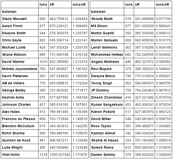
The best batsmen according to the updated metric is once again Glenn Maxwell followed by Aaron Finch.  However, Darren Sammy, who was previously in 3rd position, has dropped all the way to 33rd.  This is a reflection of his under-performance in scoring runs near the end of the innings.  This may also be true of MS Dhoni whose xR/runs figure drops from 1.00 to 0.889 – the equivalent of about 76 runs.  Dhoni is a great finisher of an innings but perhaps picks the right ball to hit a little too conservatively.

An example of a batsman who sees an increase in their runs/xR multiple is David Warner, from 1.14 to 1.21 – the equivalent of 56 extra runs.  This perhaps illustrates the fact that he performs better in the first few overs of the innings than other openers and top-order batsmen.  If you look at the first graph above, you’ll see that of the first 12 overs of an innings, only 3 (overs 4, 5 and 6) are above the average run rate of about 7.  This means batting in this period will result in your xR to be discounted as it were.  Other examples include Aaron Finch and Chris Gayle who this updated model rates more favourably.  On the other hand, Luke Wright’s runs/xR drops ever so slightly from 1.13 to 1.12.

For bowlers with at least 200 balls, the top and bottom 10, measured by xR/ball, are shown below.  It should be noted again that spinners historically have had a lower economy rate than pace bowlers in T20 cricket.  This coupled with the fact that spinners tend to bowl in the middle overs means that this updated model favours spinners a slightly more than pace bowlers.

As expected, spinners make up the bulk of the top performers list.  The best performing fast bowler is South Africa’s Lonwabo Tsotsobe with an xR/ball of 1.16.  One important difference to the previous model is the fact that the xR/ball figures have all dropped for bowlers in the top 10 and increased for bowlers in the bottom 10.  Mohammad Hafeez’s xR/ball has gone from 1.08 to 1.00 while Dwayne Bravo’s has gone from 1.40 to 1.50.  This shows how the new model can be useful in identifying the best bowlers at certain stages of the innings.

Furthermore, we can see how the updated xW model affects both batsmen and bowlers.  You can see from the second graph above that the wicket rate for every over up to the 14th is below the average wicket rate, so the xW of any balls in that period will be discounted and vice versa.  The best and worst performing batsmen, with at least 15 dismissals, measured by dismissals/xW are shown below.

This time JP Duminy is top after adjusting xW for game state.  At the other end, surprisingly Shahid Afridi drops down to 4th worst with Michael Lumb taking his place.  Interestingly there are quite a few openers in the bottom 10 compared to the previous model even though this model favours batsmen who bat in the opening overs.  This possibly highlights the hit-and-miss nature for openers in T20’s.  Perhaps an extension to this model would include adjustment factors for different positions in the batting order.

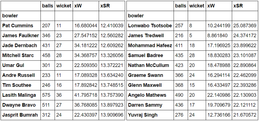
Expected Strike Rate (xSR) is calculated from the number of balls divided by xW.  In general, pace bowlers have had a lower strike rate than spinners in T20 cricket so it is not surprising to see only fast bowlers in the top 10 and mostly spinners in the bottom 10.  Tsotsobe however, who we saw previously to be the best performing pace bowler in terms of runs/xR,  has the highest xSR of any bowler.  This is consistent with his career stats which suggests he is a bowler who keeps it tight in the latter overs without getting a load of wickets.

Overall, the intuition between adding game state to the model is simple – if a player scores more runs or takes more wickets than on average at a particular stage of the innings then they deserve some credit and tells us something about their game.  I realise this article consisted of a lot of tables of data, but I’ll be sure to include some more informative graphics in the future.  In the next post I hope to look into game state further, specifically which batsmen and bowlers perform the best in the powerplay and death overs and why they’re able to do so.

Questions/suggestions?  Tweet me here.